A Technical Deep Dive into Diffusion Models: Theory, Mathematics, and Implementation (Placeholder)

1. Introduction to Diffusion Models

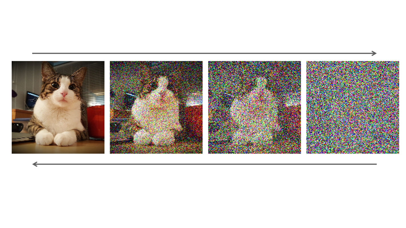
Diffusion models are based on the idea of gradually adding noise to data and then learning to reverse this process. The forward process (noise addition) is fixed, while the reverse process (noise removal) is learned. This approach allows for high-quality sample generation and offers unique advantages over other generative models like GANs and VAEs.

2. Mathematical Foundations

2.1 Forward Process

The forward process is defined as a Markov chain that gradually adds Gaussian noise to the data. Let $x_0$ be our initial data point, and $x_1, \ldots, x_T$ be the subsequent noisy versions. The forward process is defined as:

q(x_t | x_{t-1}) = \mathcal{N}(x_t; \sqrt{1 - \beta_t} x_{t-1}, \beta_t I)

where $\beta_t$ is a variance schedule that controls the amount of noise added at each step.

We can derive a useful property that allows us to sample $x_t$ directly given $x_0$ :

q(x_t | x_0) = \mathcal{N}(x_t; \sqrt{\bar{\alpha}_t} x_0, (1 - \bar{\alpha}_t) I)

where $\alpha_t = 1 - \beta_t$ and $\bar{\alpha}_t = \prod_{s=1}^t \alpha_s$ .

2.2 Reverse Process

The reverse process aims to gradually denoise the data, starting from pure noise $x_T$ and working backwards to recover the original data $x_0$ . We model this process as:

p_\theta(x_{t-1} | x_t) = \mathcal{N}(x_{t-1}; \mu_\theta(x_t, t), \Sigma_\theta(x_t, t))

where $\mu_\theta$ and $\Sigma_\theta$ are learned functions parameterized by $\theta$ .

2.3 Variational Lower Bound

To train the model, we optimize a variational lower bound on the log-likelihood:

$\mathcal{L} = \mathbb{E}_{q(x_0)} \left[ -\log p_\theta(x_0) \right] \leq \mathbb{E}_{q(x_{0:T})} \left[ \log \frac{q(x_{1:T} | x_0)}{p_\theta(x_{0:T})} \right]$

This can be further decomposed into:

\mathcal{L} = \mathcal{L}_0 + \mathcal{L}_1 + \ldots + \mathcal{L}_T

where:

\mathcal{L}_t = \mathbb{E}_{q} \left[ D_{KL}(q(x_{t-1} | x_t, x_0) || p_\theta(x_{t-1} | x_t)) \right] \quad \text{for } t > 1

\mathcal{L}_0 = \mathbb{E}_{q} \left[ -\log p_\theta(x_0 | x_1) \right]

\mathcal{L}_T = \mathbb{E}_{q} \left[ D_{KL}(q(x_T | x_0) || p(x_T)) \right]

3. Training Objective

The primary training objective is to minimize the reverse KL divergence:

$\min_\theta \mathbb{E}_{t, x_0, \epsilon} \left[ \| \epsilon - \epsilon_\theta(x_t, t) \|^2 \right]$

where $\epsilon \sim \mathcal{N}(0, I)$ and $x_t = \sqrt{\bar{\alpha}_t} x_0 + \sqrt{1 - \bar{\alpha}_t} \epsilon$ .

This objective is derived from the fact that the optimal reverse process satisfies:

$\mu_\theta^*(x_t, t) = \frac{1}{\sqrt{\alpha_t}} \left( x_t - \frac{\beta_t}{\sqrt{1 - \bar{\alpha}_t}} \epsilon_\theta(x_t, t) \right)$

4. PyTorch Implementation

Let's implement key components of a diffusion model using PyTorch.

4.1 Noise Schedule

First, we'll define the noise schedule:

import torch
import torch.nn as nn
 
class NoiseSchedule(nn.Module):
    def __init__(self, num_timesteps):
        super().__init__()
        self.num_timesteps = num_timesteps
        
        # Linear schedule from Ho et al. (2020)
        beta_start = 1e-4
        beta_end = 2e-2
        self.betas = torch.linspace(beta_start, beta_end, num_timesteps)
        self.alphas = 1 - self.betas
        self.alpha_bars = torch.cumprod(self.alphas, dim=0)
 
    def forward(self, t):
        return self.betas[t], self.alphas[t], self.alpha_bars[t]

4.2 U-Net Architecture

Next, we'll implement a simplified U-Net architecture, which is commonly used as the backbone for diffusion models:

class ResidualBlock(nn.Module):
    def __init__(self, in_channels, out_channels):
        super().__init__()
        self.conv1 = nn.Conv2d(in_channels, out_channels, 3, padding=1)
        self.conv2 = nn.Conv2d(out_channels, out_channels, 3, padding=1)
        self.bn1 = nn.BatchNorm2d(out_channels)
        self.bn2 = nn.BatchNorm2d(out_channels)
        self.relu = nn.ReLU()
        
        if in_channels != out_channels:
            self.shortcut = nn.Conv2d(in_channels, out_channels, 1)
        else:
            self.shortcut = nn.Identity()
 
    def forward(self, x):
        residual = x
        x = self.relu(self.bn1(self.conv1(x)))
        x = self.bn2(self.conv2(x))
        x += self.shortcut(residual)
        x = self.relu(x)
        return x
 
class UNet(nn.Module):
    def __init__(self, in_channels, out_channels, time_emb_dim=256):
        super().__init__()
        
        # Time embedding
        self.time_mlp = nn.Sequential(
            nn.Linear(1, time_emb_dim),
            nn.ReLU(),
            nn.Linear(time_emb_dim, time_emb_dim)
        )
        
        # Encoder
        self.enc1 = ResidualBlock(in_channels + time_emb_dim, 64)
        self.enc2 = ResidualBlock(64, 128)
        self.enc3 = ResidualBlock(128, 256)
        
        # Bottleneck
        self.bottleneck = ResidualBlock(256, 512)
        
        # Decoder
        self.dec3 = ResidualBlock(512 + 256, 256)
        self.dec2 = ResidualBlock(256 + 128, 128)
        self.dec1 = ResidualBlock(128 + 64, 64)
        
        self.final = nn.Conv2d(64, out_channels, 1)
        
        self.maxpool = nn.MaxPool2d(2)
        self.upsample = nn.Upsample(scale_factor=2, mode='bilinear', align_corners=False)
 
    def forward(self, x, t):
        # Time embedding
        t_emb = self.time_mlp(t.unsqueeze(-1)).unsqueeze(-1).unsqueeze(-1)
        t_emb = t_emb.expand(-1, -1, x.shape[2], x.shape[3])
        
        # Encoder
        x1 = self.enc1(torch.cat([x, t_emb], dim=1))
        x2 = self.enc2(self.maxpool(x1))
        x3 = self.enc3(self.maxpool(x2))
        
        # Bottleneck
        x = self.bottleneck(self.maxpool(x3))
        
        # Decoder
        x = self.upsample(x)
        x = self.dec3(torch.cat([x, x3], dim=1))
        x = self.upsample(x)
        x = self.dec2(torch.cat([x, x2], dim=1))
        x = self.upsample(x)
        x = self.dec1(torch.cat([x, x1], dim=1))
        
        return self.final(x)

4.3 Diffusion Model

Now, let's implement the main diffusion model:

class DiffusionModel(nn.Module):
    def __init__(self, unet, noise_schedule):
        super().__init__()
        self.unet = unet
        self.noise_schedule = noise_schedule
 
    def forward(self, x, t):
        return self.unet(x, t)
 
    def loss(self, x_0):
        batch_size = x_0.shape[0]
        t = torch.randint(0, self.noise_schedule.num_timesteps, (batch_size,), device=x_0.device)
        
        noise = torch.randn_like(x_0)
        x_t = self.q_sample(x_0, t, noise)
        
        predicted_noise = self(x_t, t)
        
        loss = nn.MSELoss()(noise, predicted_noise)
        return loss
 
    def q_sample(self, x_0, t, noise):
        _, _, alpha_bar = self.noise_schedule(t)
        alpha_bar = alpha_bar.view(-1, 1, 1, 1)
        
        x_t = torch.sqrt(alpha_bar) * x_0 + torch.sqrt(1 - alpha_bar) * noise
        return x_t
 
    @torch.no_grad()
    def p_sample(self, x_t, t):
        beta, alpha, alpha_bar = self.noise_schedule(t)
        beta = beta.view(-1, 1, 1, 1)
        alpha = alpha.view(-1, 1, 1, 1)
        alpha_bar = alpha_bar.view(-1, 1, 1, 1)
        
        predicted_noise = self(x_t, t)
        
        mean = (1 / torch.sqrt(alpha)) * (x_t - (beta / torch.sqrt(1 - alpha_bar)) * predicted_noise)
        var = beta
        
        epsilon = torch.randn_like(x_t)
        return mean + torch.sqrt(var) * epsilon
 
    @torch.no_grad()
    def sample(self, num_samples, img_shape):
        device = next(self.parameters()).device
        x_T = torch.randn((num_samples, *img_shape), device=device)
        
        for t in reversed(range(self.noise_schedule.num_timesteps)):
            t_batch = torch.full((num_samples,), t, device=device, dtype=torch.long)
            x_T = self.p_sample(x_T, t_batch)
        
        return x_T

5. Training Loop

Here's a basic training loop for our diffusion model:

def train(model, dataloader, optimizer, num_epochs):
    for epoch in range(num_epochs):
        for batch in dataloader:
            optimizer.zero_grad()
            loss = model.loss(batch)
            loss.backward()
            optimizer.step()
        print(f"Epoch {epoch + 1}, Loss: {loss.item():.4f}")
 
# Instantiate the model and optimizer
unet = UNet(in_channels=3, out_channels=3)
noise_schedule = NoiseSchedule(num_timesteps=1000)
model = DiffusionModel(unet, noise_schedule)
optimizer = torch.optim.Adam(model.parameters(), lr=1e-4)
 
# Train the model
train(model, dataloader, optimizer, num_epochs=100)

6. Advanced Topics

6.1 Improved Sampling Techniques

Several techniques have been proposed to improve the sampling process:

DDIM (Denoising Diffusion Implicit Models): This technique allows for faster sampling by skipping steps in the reverse process.
Classifier guidance: By incorporating a pre-trained classifier, we can guide the generation process towards specific classes or attributes.
Adaptive step size: Dynamically adjusting the step size during sampling can lead to faster and higher-quality generation.

6.2 Continuous Time Formulation

Recent work has explored formulating diffusion models in continuous time, leading to more flexible and theoretically grounded models. The stochastic differential equation (SDE) formulation is given by:

$dx = f(x, t)dt + g(t)dW$

where $f(x, t)$ is the drift coefficient, $g(t)$ is the diffusion coefficient, and $W$ is a Wiener process.

The corresponding reverse-time SDE is:

$dx = [f(x, t) - g(t)^2 \nabla_x \log p_t(x)]dt + g(t)d\bar{W}$

where $\bar{W}$ is a reverse-time Wiener process.

6.3 Score-Based Generative Models

Score-based generative models provide an alternative perspective on diffusion models. They focus on estimating the score function $\nabla_x \log p(x)$ rather than directly modeling the probability density. This approach leads to a unified framework that encompasses both diffusion models and noise-conditioned score networks.